Tutorial

This tutorial follows the paper “Angular velocity of gravitational radiation from precessing binaries and the corotating frame,” giving examples of the code relevant to each of its sections. The section numbers below refer to the paper. Every code cell on this page is run whenever the documentation is built, so the outputs shown are those of the current version of GWFrames.

import numpy as np
import matplotlib.pyplot as plt

import GWFrames
from GWFrames import Quaternions

I. Introduction

The primary objects provided by GWFrames are Waveform, PNWaveform, and Quaternion. A Waveform holds the spin-weighted spherical-harmonic modes \(h^{\ell,m}(t)\) of some quantity, along with the frame in which those modes are decomposed. A PNWaveform is a Waveform computed from a post-Newtonian model of a binary, which also records the orbital quantities of that binary. A Quaternion represents a rotation, or a vector in three dimensions.

Python’s help function shows the documentation of any of these objects, as in help(GWFrames.PNWaveform); the same documentation is in the API reference.

Constructing a post-Newtonian waveform

As an example, we construct the post-Newtonian waveform of a precessing binary with a mass ratio of 6, in which both black holes are spinning. The spins are given in spherical coordinates, as a magnitude and two angles, and converted to Cartesian vectors.

def spin(magnitude, vartheta, varphi):
    return magnitude * np.array(
        [np.sin(vartheta) * np.cos(varphi), np.sin(vartheta) * np.sin(varphi), np.cos(vartheta)]
    )

m1, m2 = 6.0, 1.0
delta = (m1 - m2) / (m1 + m2)
chi1 = spin(0.9, 2.0, 0.25)
chi2 = spin(0.3, 2.4, 2.9)
Omega0 = 0.02  # The initial orbital frequency

W_PN = GWFrames.PNWaveform("TaylorT4", delta, chi1, chi2, Omega0)

The resulting waveform holds the modes at the times chosen by the integrator, with \(t=0\) when the orbital frequency is Omega0:

print(W_PN.NTimes(), "times and", W_PN.NModes(), "modes, in the", W_PN.FrameTypeString(), "frame")
print(f"The times run from {W_PN.T(0)} to {W_PN.T(W_PN.NTimes() - 1):.1f}")

18115 times and 77 modes, in the Coorbital frame
The times run from 0.0 to 3905.8

The waveform is constructed in the co-orbital frame, which follows the orbit of the binary. Most of what follows starts from the inertial frame, so we transform it there.

W_PN.TransformToInertialFrame();

The post-Newtonian approximation breaks down as the black holes approach merger, where the integration stops. The last few time steps are therefore not physically meaningful, and their values are large enough to swamp everything else in a plot. The plots below show only the inspiral, ending \(100M\) before the end of the data.

def inspiral(T, margin=100.0):
    """Return a mask selecting the times more than `margin` before the last"""
    T = np.asarray(T)
    return T < T[-1] - margin

I = inspiral(W_PN.T())

A Waveform can also be read from a data file. In a text file, the first column holds the time, and the following columns hold the magnitude and phase of each mode in turn (or its real and imaginary parts, with "ReIm" instead of "MagArg"). The modes are assumed to be in the order \((2,-2), (2,-1), \ldots\); if they are not, they must be reordered manually. The functions GWFrames.ReadFromH5 and GWFrames.ReadFromNRAR read HDF5 files.

W_NR = GWFrames.Waveform("/path/to/data/rhOverM.dat", "MagArg")

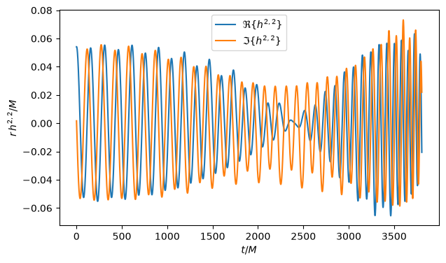
The modes are accessed by index, which FindModeIndex finds from \((\ell, m)\):

i22 = W_PN.FindModeIndex(2, 2)
fig, ax = plt.subplots()
ax.plot(W_PN.T()[I], W_PN.Re(i22)[I], label=r"$\Re\{h^{2,2}\}$")
ax.plot(W_PN.T()[I], W_PN.Im(i22)[I], label=r"$\Im\{h^{2,2}\}$")
ax.set_xlabel(r"$t/M$")
ax.set_ylabel(r"$r\, h^{2,2} / M$")
ax.legend();

Quaternion notation

A Quaternion can be constructed from its four components:

Q1 = Quaternions.Quaternion(3, 1, 4, 1)
Q2 = Quaternions.Quaternion(5.9, 2.6, 5.3, 5.8)
print(Q1.conjugate())
print(Q1.abs())

[3, -1, -4, -1]
5.196152422706632

A vector is a quaternion with zero scalar part, and a rotor (a unit quaternion) \(R\) rotates a vector \(\vec{v}\) to \(R\, \vec{v}\, \bar{R}\). Here, we construct \(\hat{z}\) and rotate it by an angle \(\pi/2\) about the \(x\) axis, which gives \(-\hat{y}\) (up to roundoff):

z = Quaternions.Quaternion([0, 0, 1])
R = Quaternions.exp((np.pi / 2) * Quaternions.Quaternion([1, 0, 0]) / 2)
R * z * R.conjugate()

Quaternion(0, 0, -1, 1.79380389039135e-16)

The rotor was defined with the quaternion exponential. Its logarithm recovers the vector \((\pi/4)\, \hat{x}\):

Quaternions.log(R)

Quaternion(0, 0.785398163397448, 0, 0)

II. Angular velocity of a waveform

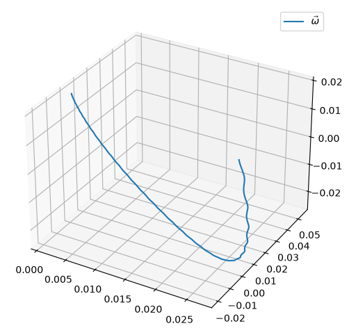
The angular velocity of a waveform is computed from its modes alone, by AngularVelocityVector. By default, all values of \(\ell\) are used; a PNWaveform has modes with \(2 \leq \ell \leq 8\).

omega = W_PN.AngularVelocityVector()

fig = plt.figure(figsize=(6, 6))
ax = fig.add_subplot(projection="3d")
ax.plot(*omega[I].T, label=r"$\vec{\omega}$")
ax.legend();

III. Solving the inverse problem

A PNWaveform records the orbital and precessional angular velocities of the binary that produced it. We can compare them to quantities measured from the waveform data alone: the dominant eigenvector \(\hat{V}_h\) of \(\langle L L \rangle\), and the angular velocity \(\vec{\omega}\). The following reproduces Fig. 1 of the paper.

OmegaHat_orb = W_PN.OmegaHat_orb()
VHat_h = W_PN.LLDominantEigenvector()
Omega_tot = W_PN.Omega_tot()

fig = plt.figure(figsize=(10, 5))
ax = fig.add_subplot(1, 2, 1, projection="3d")
ax.plot(*OmegaHat_orb[I].T, lw=1, label=r"$\hat{\Omega}_{\mathrm{orb}}$")
ax.plot(*VHat_h[I].T, ls="--", lw=2, label=r"$\hat{V}_{h}$")
ax.legend()
ax = fig.add_subplot(1, 2, 2, projection="3d")
ax.plot(*Omega_tot[I].T, lw=1, label=r"$\vec{\Omega}_{\mathrm{tot}}$")
ax.plot(*omega[I].T, ls="--", lw=2, label=r"$\vec{\omega}$")
ax.legend();

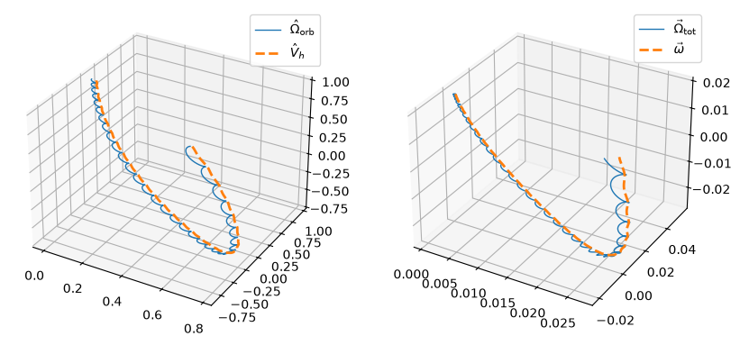
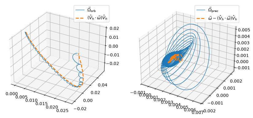
The component of \(\vec{\omega}\) along \(\hat{V}_h\) is the “PN-equivalent” orbital angular velocity, and the remainder is the PN-equivalent precessional angular velocity. The orbital parts agree closely. The precessional parts are smaller by roughly an order of magnitude, and they agree less well.

Omega_orb = W_PN.Omega_orb()
Omega_prec = W_PN.Omega_prec()
OrbitalAV_equiv = np.sum(VHat_h * omega, axis=1)[:, np.newaxis] * VHat_h
PrecessionalAV_equiv = omega - OrbitalAV_equiv

fig = plt.figure(figsize=(10, 5))
ax = fig.add_subplot(1, 2, 1, projection="3d")
ax.plot(*Omega_orb[I].T, lw=1, label=r"$\vec{\Omega}_{\mathrm{orb}}$")
ax.plot(*OrbitalAV_equiv[I].T, ls="--", lw=2, label=r"$(\hat{V}_{h} \cdot \vec{\omega}) \hat{V}_{h}$")
ax.legend()
ax = fig.add_subplot(1, 2, 2, projection="3d")
ax.plot(*Omega_prec[I].T, lw=1, label=r"$\vec{\Omega}_{\mathrm{prec}}$")
ax.plot(*PrecessionalAV_equiv[I].T, ls="--", lw=2,
        label=r"$\vec{\omega} - (\hat{V}_{h} \cdot \vec{\omega}) \hat{V}_{h}$")
ax.legend();

IV. The corotating frame

A. Finding the corotating frame

The corotating frame is the frame whose angular velocity is \(\vec{\omega}\). Given the angular velocity as a function of time, FrameFromAngularVelocity integrates it to find the rotors \(R_{\mathrm{corot}}(t)\) of that frame. (The methods shown in the next section do this and transform the waveform in one step.)

R_corot = Quaternions.FrameFromAngularVelocity(Quaternions.QuaternionArray(omega), W_PN.T())

The system starts out rotating mostly about the \(z\) axis, because of the orbital motion, but it also precesses a little. The frame at the third time step has been rotated about an axis that is nearly parallel to \(z\), with a small \(x\) component. The angle of that rotation is about what we expect from the initial orbital frequency of 0.02:

Rotor = R_corot[2]
Angle = Rotor.angle()
Axis = np.array(Rotor.log().vec()) * (2 / Angle)
Time = W_PN.T(2) - W_PN.T(0)
print(f"Time   = {Time:.4f} M after the beginning")
print(f"Rotor  = {Rotor}")
print(f"Axis   = {Axis}")
print(f"Angle  = {Angle:.6f}")
print(f"Ω₀ × t = {Omega0 * Time:.6f}")

Time   = 0.3247 M after the beginning
Rotor  = [0.999994716889527, 0.000154257792338604, 1.90465524255333e-05, 0.00324684998060061]
Axis   = [0.04745564 0.00585945 0.99885616]
Angle  = 0.006501
Ω₀ × t = 0.006494

B. Gravitational waveforms in the corotating frame

Rather than computing the angular velocity, then the frame, and then transforming the modes, we can use the TransformTo... methods, which do all of these at once. Each of them changes the waveform in place, so we transform copies, which the PNWaveform constructor makes from another PNWaveform. (Plain assignment in Python makes a new reference to the same object, not a copy.)

W_PN_Coprec = GWFrames.PNWaveform(W_PN)
W_PN_Coprec.TransformToCoprecessingFrame()
W_PN_Corot = GWFrames.PNWaveform(W_PN)
W_PN_Corot.TransformToCorotatingFrame();

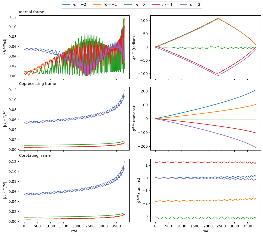
In the inertial frame, the modes oscillate rapidly and their amplitudes are modulated by the precession. In the coprecessing frame, the amplitudes are nearly monotonic, but the phases still increase rapidly. In the corotating frame, both the amplitudes and the phases vary slowly.

def plot_ell_2_modes(axes, W, title):
    I = inspiral(W.T())
    for m in range(-2, 3):
        i = W.FindModeIndex(2, m)
        axes[0].plot(W.T()[I], W.Abs(i)[I], label=f"$m={m}$")
        axes[1].plot(W.T()[I], W.ArgUnwrapped(i)[I])
    axes[0].set_ylabel(r"$|r\, h^{2,m}/M|$")
    axes[1].set_ylabel(r"$\phi^{2,m}$ (radians)")
    axes[0].set_title(title, loc="left", fontsize="medium")

fig, axes = plt.subplots(3, 2, figsize=(10, 9), sharex=True, layout="constrained")
plot_ell_2_modes(axes[0], W_PN, "Inertial frame")
plot_ell_2_modes(axes[1], W_PN_Coprec, "Coprecessing frame")
plot_ell_2_modes(axes[2], W_PN_Corot, "Corotating frame")
fig.legend(*axes[0, 0].get_legend_handles_labels(), loc="outside upper center", ncol=5)
for ax in axes[2]:
    ax.set_xlabel(r"$t/M$")

C. Comparison, alignment, and hybridization

Any two waveforms can be compared, aligned, and hybridized. As an example, we construct a second waveform for the same binary, but with the spins given at a slightly lower orbital frequency, so that the two waveforms differ slightly.

W_A = GWFrames.PNWaveform(W_PN)
W_B = GWFrames.PNWaveform("TaylorT4", delta, chi1, chi2, 0.999 * Omega0)
W_B.TransformToInertialFrame();

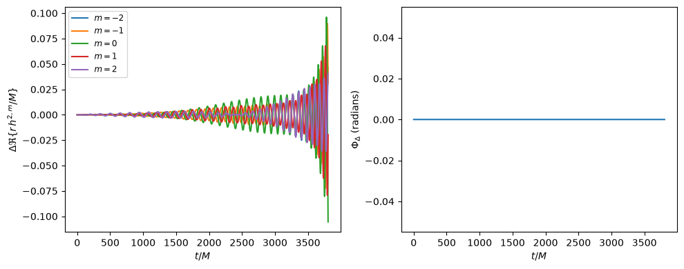
Compare returns a Waveform holding the differences between the modes of the two waveforms, and the rotors taking one frame to the other. Here both frames are inertial, so the frames agree, but the modes differ considerably because the two waveforms drift out of phase.

def plot_differences(W_A, W_B):
    W_diff = W_A.Compare(W_B)
    I = inspiral(W_diff.T())
    fig, axes = plt.subplots(1, 2, figsize=(10, 4))
    for m in range(-2, 3):
        axes[0].plot(W_diff.T()[I], W_diff.Re(W_diff.FindModeIndex(2, m))[I], label=f"$m={m}$")
    axes[0].set_ylabel(r"$\Delta \Re\{r\, h^{2,m}/M\}$")
    axes[0].legend(fontsize="small")
    # The frame is empty when it is constant and equal to the identity
    angles = np.array([R.angle() for R in W_diff.Frame()]) if len(W_diff.Frame()) else 0.0
    axes[1].plot(W_diff.T()[I], np.broadcast_to(angles, (W_diff.NTimes(),))[I])
    axes[1].set_ylabel(r"$\Phi_{\Delta}$ (radians)")
    for ax in axes:
        ax.set_xlabel(r"$t/M$")
    fig.tight_layout()

plot_differences(W_A, W_B)

AlignWaveforms aligns the two waveforms over an interval of time. It transforms both of them to their corotating frames, aligns the frames to the modes, and then optimizes a time offset \(\delta t\) and a constant rotation \(R_\delta\) applied to the second waveform, so as to minimize

\[ \int_{t_1}^{t_2} \left| \log \left[ R_{\mathrm{A}}(t)\, \bar{R}_{\mathrm{B}}(t+\delta t)\, \bar{R}_\delta \right] \right|^2\, dt. \]

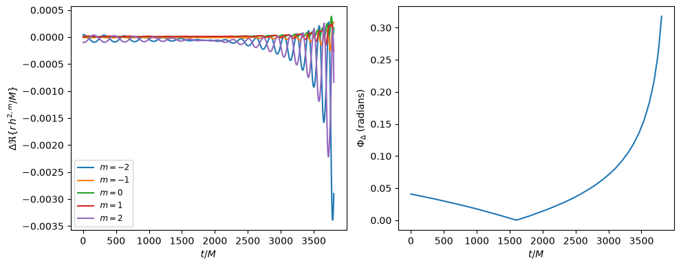
Afterward, the modes are much more nearly equal, and the frames agree closely over the alignment interval.

t1, t2 = 1500.0, 1700.0
GWFrames.AlignWaveforms(W_A, W_B, t1, t2)

plot_differences(W_A, W_B)

Appendix A. Quaternions and rotations

1. Elements of quaternion mathematics

We create a quaternion with the (arbitrary) components \((1, 2, 3, 5)\), and take its conjugate:

Q = Quaternions.Quaternion(1, 2, 3, 5)
Q.conjugate()

Quaternion(1, -2, -3, -5)

We can multiply it by another quaternion, but the product is not commutative in general:

Q2 = Quaternions.Quaternion(7, 11, 13, 17)
print(Q * Q2)
print(Q2 * Q)

[-139, 11, 55, 45]
[-139, 39, 13, 59]

The norm of a quaternion is \(\sqrt{Q \bar{Q}}\), which is also given by abs:

print(Quaternions.sqrt(Q * Q.conjugate()))
print(Q.abs())

[6.2449979983984, 0, 0, 0]
6.244997998398398

The inverse of a quaternion is its conjugate divided by its squared norm, so their product is 1 (up to roundoff):

Qinv = Q.conjugate() / Q.normsquared()
Q * Qinv

Quaternion(1, 5.55111512312578e-17, -1.38777878078145e-17, 6.93889390390723e-18)

Normalizing a quaternion gives a unit quaternion, which is a rotor:

R = Q.normalized()
R.abs()

1.0

The basis vectors are quaternions with zero scalar part, which are also available as Quaternions.xHat, Quaternions.yHat, and Quaternions.zHat. They let us construct a rotor from an axis and an angle. The following is a rotation through the angle \(\pi/2\) about the \(x\) axis, which rotates \(\hat{y}\) to \(\hat{z}\), and \(\hat{z}\) to \(-\hat{y}\):

x = Quaternions.Quaternion(0, 1, 0, 0)
y = Quaternions.Quaternion(0, 0, 1, 0)
z = Quaternions.Quaternion(0, 0, 0, 1)

theta = np.pi / 2
R = Quaternions.exp(theta * x / 2)
print(R)
print(R * y * R.conjugate())
print(R * z * R.conjugate())

[0.707106781186548, 0.707106781186547, 0, 0]
[0, 0, 1.99673461754274e-16, 1]
[0, 0, -1, 1.79380389039135e-16]

The logarithm inverts the exponential:

R.log()

Quaternion(0, 0.785398163397448, 0, 0)

However, as with the complex logarithm, there is a branch cut. For example, adding \(2\pi\, \hat{x}\) to the argument of the exponential gives the same rotor \(R\) as above, so the logarithm of the result is that of \(R\), not the argument of the exponential:

R2 = Quaternions.exp(theta * x / 2 + 2 * np.pi * x)
print(R2)
print(R2.log())

[0.707106781186548, 0.707106781186547, 0, 0]
[0, 0.785398163397448, 0, 0]

3. Integrating the angular velocity

The function Quaternions.FrameFromAngularVelocity, used in Sec. IV A, is used throughout the code to find the frame that rotates with a given angular velocity. For example, Waveform.TransformToCorotatingFrame uses the frame

R_corot = Quaternions.FrameFromAngularVelocity(
    Quaternions.QuaternionArray(W_PN.AngularVelocityVector()), W_PN.T()
)

The angular velocity is converted to an array of quaternions first, because arrays of floats are accepted as quaternions only with four components in each row.

4. Interpolation

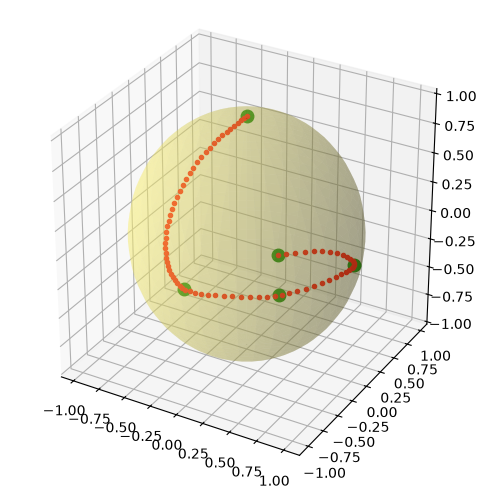
Rotations should be interpolated smoothly. Quaternions.Squad interpolates a series of rotors to new times. Here, we construct five rotors at irregularly spaced times, interpolate them to many finer steps, and plot the images of the north pole under all of these rotations. The original five points are shown as large green dots, and the interpolated points as small red dots, which follow a smooth path through the original points.

qIn = [
    Quaternions.exp((0.0 / 2) * x),
    Quaternions.exp((np.pi / 2 / 2) * x),
    Quaternions.exp((np.pi / 2 / 2) * (x + y).normalized()),
    Quaternions.exp((np.pi / 2 / 2) * y),
    Quaternions.exp((8 * np.pi / 20 / 2) * (x + y).normalized()),
]
tIn = [-10.0, 5.0, 10.0, 15.0, 20.0]
tOut = np.linspace(tIn[0], tIn[-1], 80)
qOut = Quaternions.Squad(qIn, tIn, tOut)

vartheta, varphi = np.meshgrid(np.linspace(0, np.pi, 40), np.linspace(0, 2 * np.pi, 40))
fig = plt.figure(figsize=(6, 6))
ax = fig.add_subplot(projection="3d")
ax.plot_surface(
    0.98 * np.sin(vartheta) * np.cos(varphi), 0.98 * np.sin(vartheta) * np.sin(varphi), 0.98 * np.cos(vartheta),
    color="#fff46f", alpha=0.3, linewidth=0,
)
PointsIn = np.array([(R * z * R.conjugate()).vec() for R in qIn])
PointsOut = np.array([(R * z * R.conjugate()).vec() for R in qOut])
ax.plot(*PointsIn.T, "go", ms=9)
ax.plot(*PointsOut.T, "ro", ms=3)
ax.set_box_aspect((1, 1, 1));

Appendix B. Rotating spin-weighted functions

The TransformTo... methods are the most convenient way to transform a Waveform to a particular frame. More generally, RotateDecompositionBasis rotates the basis in which the modes are decomposed by a given rotor, or by a rotor at each time step. Rotating the inertial-frame waveform by the corotating frame found above gives the same modes as Waveform.TransformToCorotatingFrame did, up to roundoff:

W_C = GWFrames.PNWaveform(W_PN)
W_C.RotateDecompositionBasis(R_corot)
print(np.max(np.abs(W_C.Data() - W_PN_Corot.Data())))

0.0

Appendix C. Other methods of choosing a frame

1. and 2. The coprecessing frame

The coprecessing frame, shown in Sec. IV B, has its \(z\) axis along the dominant eigenvector \(\hat{V}_h\) of \(\langle L L \rangle\), which is the direction that maximizes the magnitude of the \((2, \pm 2)\) modes.

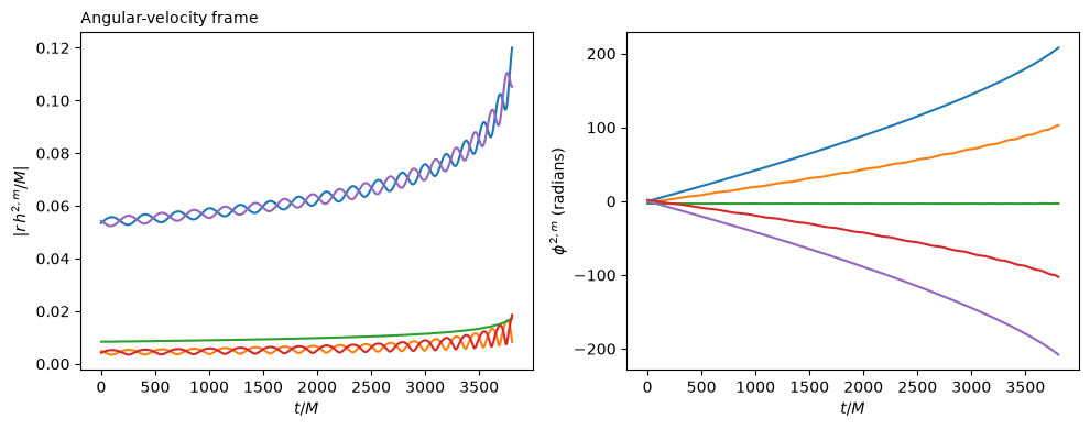
3. Aligned with the angular velocity

Another choice is the frame whose \(z\) axis is along the angular velocity \(\vec{\omega}\):

W_PN_AV = GWFrames.PNWaveform(W_PN)
W_PN_AV.TransformToAngularVelocityFrame()

fig, axes = plt.subplots(1, 2, figsize=(10, 4))
plot_ell_2_modes(axes, W_PN_AV, "Angular-velocity frame")
for ax in axes:
    ax.set_xlabel(r"$t/M$")
fig.tight_layout()

4. The minimal-rotation condition

Each of these frames specifies only the direction of its \(z\) axis. The rotation about that axis is chosen to satisfy the minimal-rotation condition, which Quaternions.MinimalRotation imposes on any series of rotors. The frame it returns has the same \(z\) axis as the input frame, but no rotation about that axis beyond what the motion of the axis requires.

R_min = Quaternions.MinimalRotation(R_corot, W_PN.T())
z_corot = np.array([(R * z * R.conjugate()).vec() for R in R_corot])
z_min = np.array([(R * z * R.conjugate()).vec() for R in R_min])
print(np.max(np.abs(z_corot - z_min)))

7.771561172376096e-16